Gravity Solver Optimisation
This document will outline the results of optimisations on the gravity solver performed by a team of scientists consisting of Dr. John Regan and Dr. Stefan Arridge from Maynooth University and Sophie Wenzel-Teuber and Dr. Buket Benek Gursoy from the Irish Centre for High End Computing (ICHEC, part of NUI Galway).
Summary
We investigated test problems with 16^3, 32^3, 64^3, 256^3 root grid, varying
number of blocks and number of PEs, with/without AMR, for around 200 cycles.
Furthermore, we analysed the bottleneck of the simulations with a
profiler and present a runtime analysis. Specifically, for dark-matter-only
cosmology runs, and 256^3 unigrid, the optimal setup was found to be 8^3
blocks, each of size 32^3. The effects of changing parameters such as
min_level and the number of V-cycles on code performance were also analysed.
It was observed that it is unlikely to achieve much speed-up just from changing
some parameters in the configuration file.
A new feature was implemented in the code to allow refresh operations to have
different values for min_face_rank and by using a smaller ghost_depth a
decrease in runtime of 30% could be achieved for a unigrid simulation.
Profiling with Projections
Charm++ has the possibility to gather tracing data of all entry functions and a visualisation tool called Projections.
The tracing data logs which processes executes which entry function at which
point in time and for how long. This creates one log file per PE. The size of
these log files can be set with the +logsize parameter.
Whenever this size is exceeded the logs are flushed to disk. This I/O can
heavily influence the tracing results as it will appear as a long execution of
an entry function in the data.
The Projections visualisation tool provides many possibilities to view this tracing data. The following image is a screenshot from a gravity simulation with 30 PEs on a grid of 64x64x64 cells, divided into 4 blocks per dimension.
All tracing and runtime measurements have been performed on ICHEC’s supercomputer on one or two nodes consisting of 40 Intel Skylake processors each and 192GiB (1.5TiB) RAM.
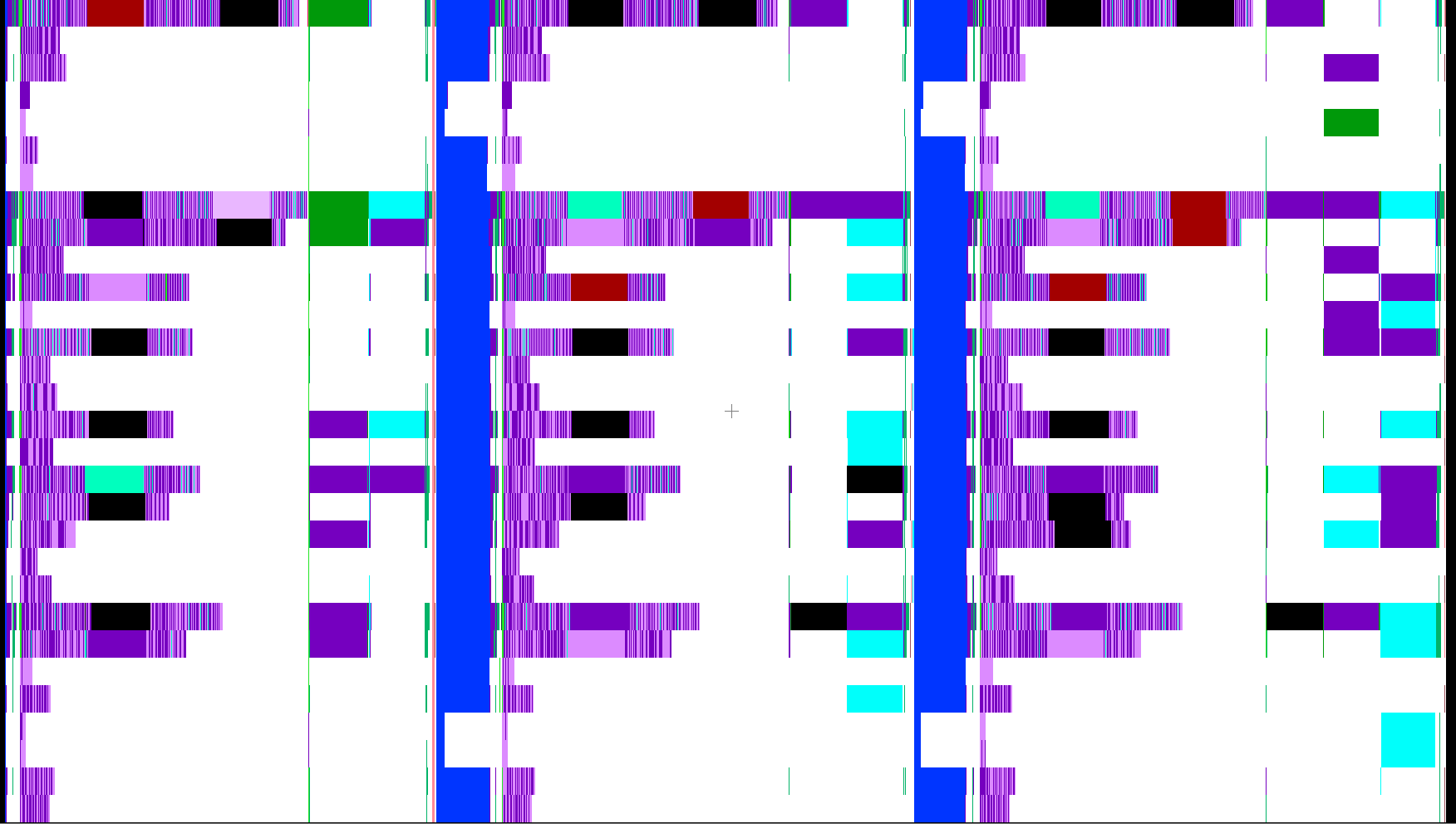
The X axis shows the time of 3 cycles (203-205) and the Y axis has one line per PE of colour codes for the entry functions this PE executed. White signals idle time.
The purple coloured lines are the refresh routine (functions
p_dot_recv_children in the brighter and p_new_refresh_recv in the
darker shade).
The blue columns represent the r_stopping_compute_timestep function and
signal the end of one and beginning of a new timestep. The equal length of this
function for almost all PEs suggest that the log data was flushed during the
execution of this function. Therefore, the execution time shown in the image is
not representable for the real runtime. The same is true for equally sized
time spans in other functions throughout the plot.
Especially the black blocks that represent “overhead” probably have to be neglected as well as this overhead almost never appears in plots without the problem of flushing log files to disk.
However, what can safely be said is that the refresh routine plays a vital role for the performance of this Enzo-E simulation.
Other plots of Projections show that the refresh routine alone accounts for more than 24 million messages in the 3 cycles above of which most result in an entry function execution time of less than 0.02s.
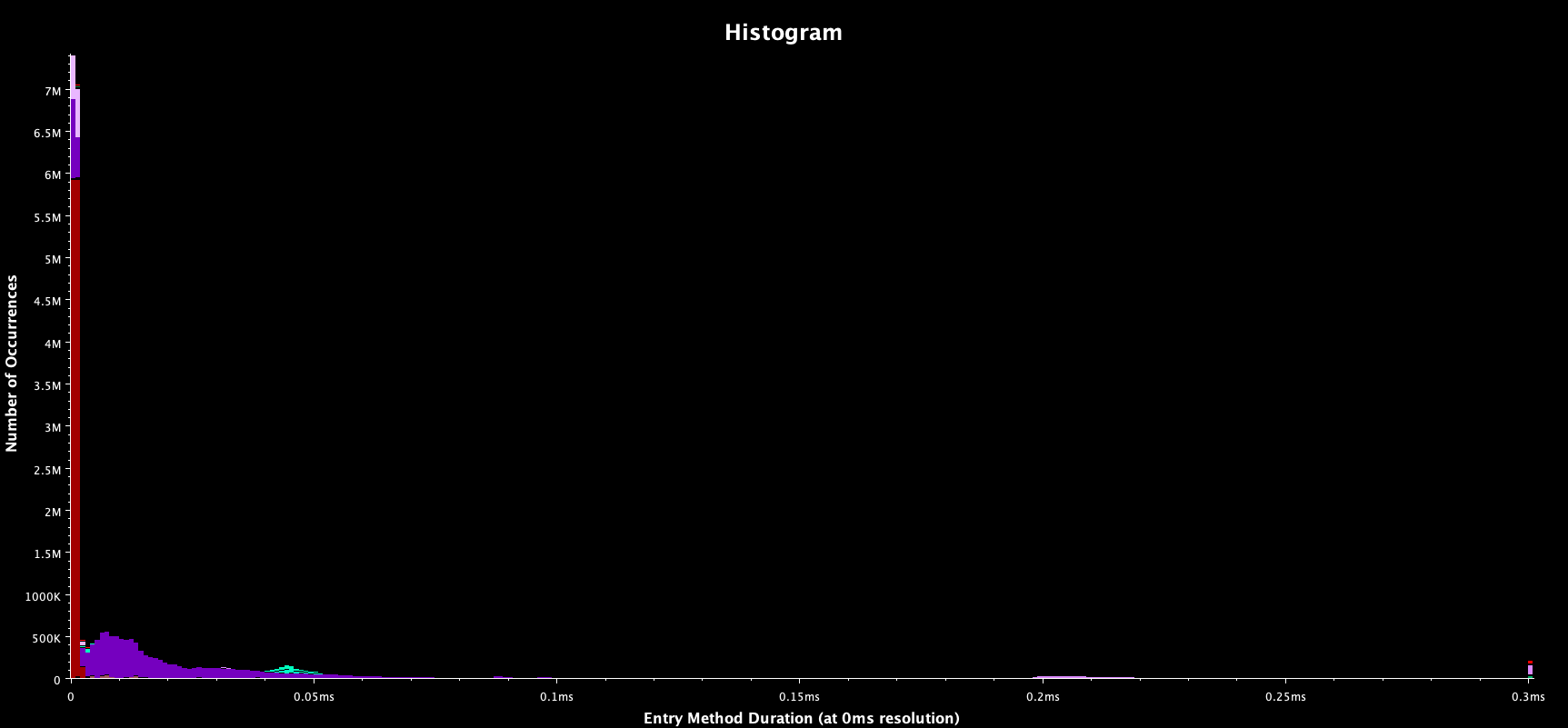
This image shows a histogram of the execution times of the messages for the entry functions.
Purple coloured are the refresh functions as above. Red represents
p_control_sync_count, which is also called in this routine to query the
refresh state of a blocks neighbours.
When disabling the adaptive mesh refinement and running in a unigrid mode the effect of the refresh routine is much smaller and the stages of the simulation can be identified in the overview.
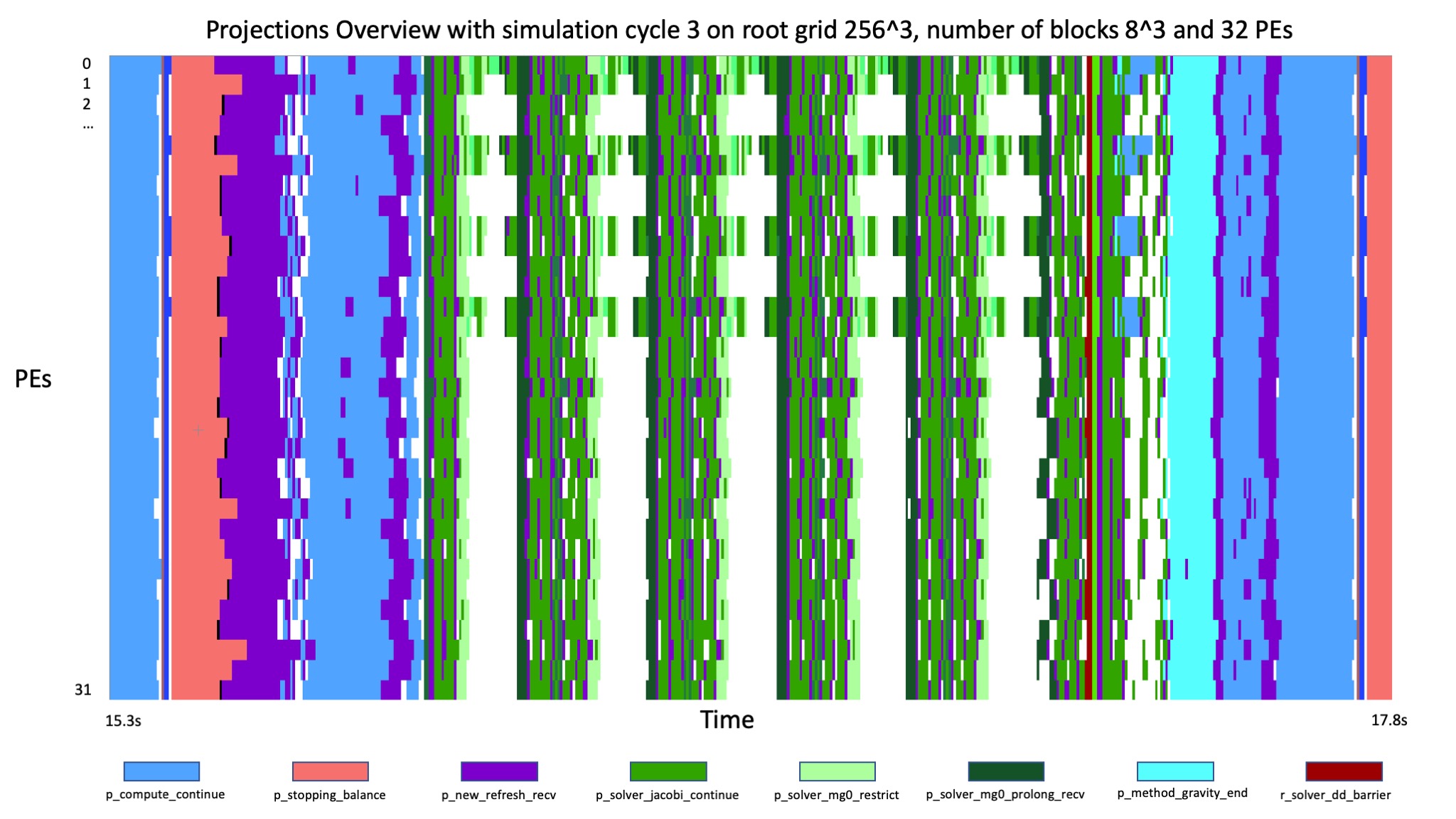
This simulation was run on a grid of 256 cells cubed, divided into 8 blocks per direction and parallelised over 32 PEs.
The five cycles of the Multigrid solver are clearly distinguishable because all
PEs except one are idle. The number of V-cycles can be adjusted in the parameter
file and will automatically reduce due to a smaller residual later in the
simulation.
Less coarsening of the grid such that more than only one processor is solving
the problem and therefore reducing the idle time of the other processors is
possible by adjusting the min_level parameter but results in longer
runtimes (presumably due to communication).
The function p_compute_continue also has a large
impact on the simulation time and is accountable for starting all solvers that
are linked to the simulation.
Runtime analysis for unigrid on a single node
To compare parameters and runtime settings in future analysis a good setup has to be found first that can yield the baseline for performance observations.
All combinations of the grid sizes 32, 64 and 256 cubed, the number of blocks of 2, 4, 8, 16, 32 and 64 per direction (where applicable) and the number of PEs of 2, 4, 8, 16, 32 and 64 (also where applicable) were run for a simulation without adaptive mesh refinement for clarity.
This provides a lot of numbers that are difficult to compare. The goal is to find metrics that cover a beneficial balance between a good workload per PE and therefore a performance utilisation of the resources, and a high parallelisation.
What was used is a mixture of weak and strong scaling:
The following plot shows the runtime per cycle (total runtime / number of
cycles) for a simulation size of 256 cubed for four constant numbers of
blocks per PE.
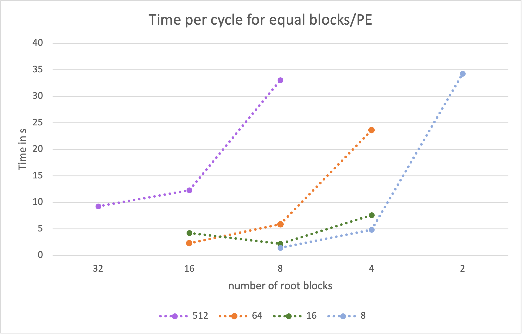
For example for a number of 64 blocks per PE the runtimes were calculated for
16^3 blocks on 64PEs
8^3 blocks on 8 PEs
4^3 blocks on 1 PE.
This means in the graph above from left to right the blocks become larger but with less parallelisation. Therefore, each PE has more to calculate on the right side of the graph than on the left, but less to communicate.
A similar plot can be created for the accumulated time of all PEs to perform one cycle - this is the value from above multiplied by the number of PEs. This relates to the CPU time needed to complete one step of the simulation.
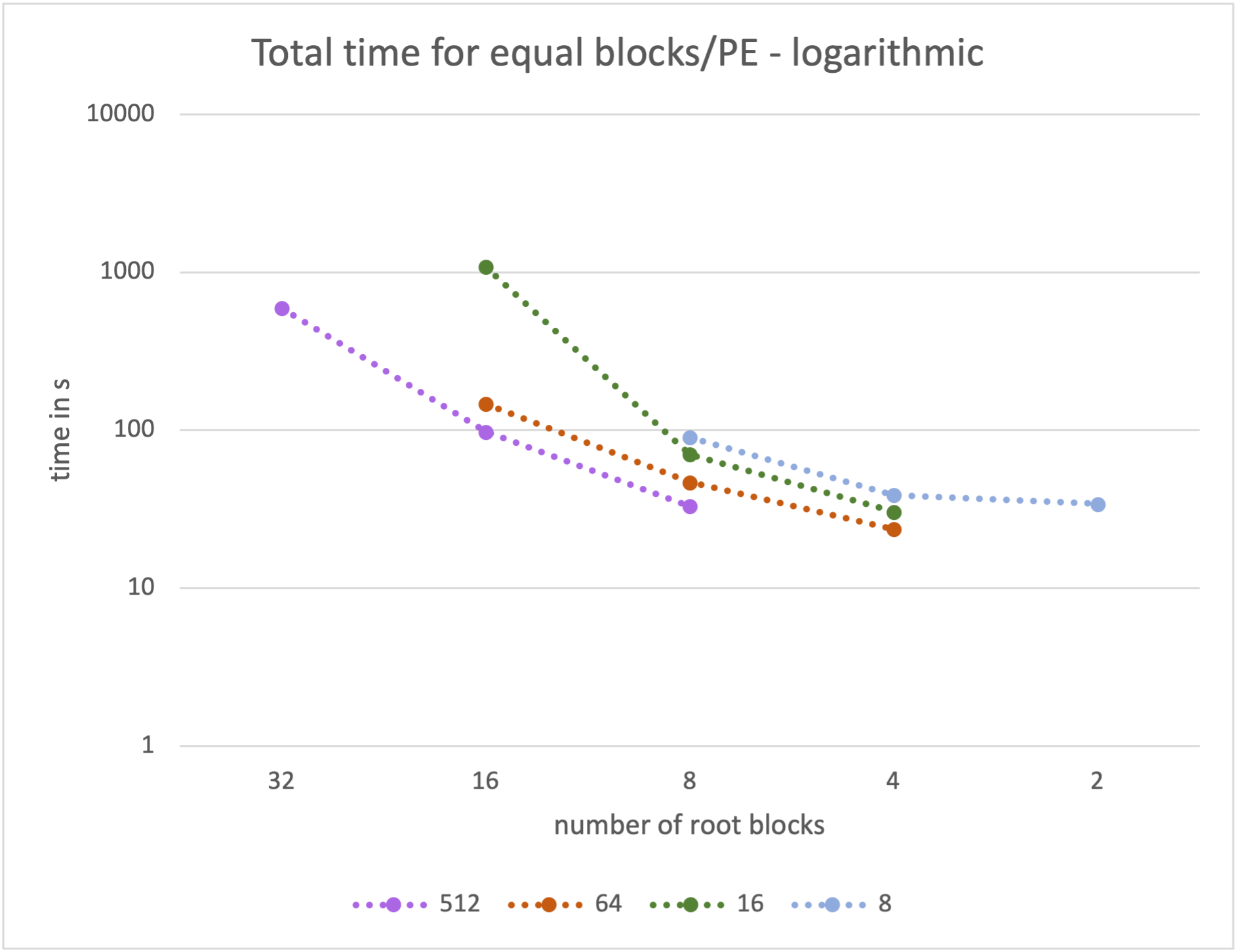
From this graph it is clear that it is more efficient to compute larger blocks on fewer PEs.
Clearly, both representations have to be combined as each one is insufficient for an educated guess of a balanced setup. From this combination we concluded that a good initial setup of the simulation for further tests is using 32PEs and 8 blocks on a grid of 256 cubed cells (which relates to the mid point of the green line in the two plots above).
These metrics fail at smaller simluation sizes for two reasons: The amount of computational work can be viewed as too small compared to the overhead and the parameter space is not sufficient to produce enough results for meaningful graphs of the metrics mentioned above. It is still the case however that fewer but larger blocks and fewer PEs result in less CPU time per cycle (again, due to the reduced overhead for communication).
Refresh routine
As mentioned above the refresh routine is the most limiting factor in a single node AMR run.
How large the ghost zones are that are copied and how many neighbours take part in the exchange is parameterised by two variables.
The ghost_depth that determines the number of cells that are copied in a
direction was set to 4 in the runs above which is a necessity at the moment.
Significant code changes would be required to adapt this value for the
distinctive refresh routines started by the different parts of Enzo-E.
Only in a simulation on a uniform grid this value can be decreased. Comparing the runtime of simulations with a ghost depth of 2 and 4 resulted in a decrease from 2.7872s to 2.1578s (speedup of 1.292) for a simulation with the setting determined in the method above (256^3 cells in 8^3 blocks and 32 PEs).
Another parameter are the number of neighbours that exchange their ghost zones. In a three dimensional grid a cell has 26 neighbours. 6 of them share a face, 12 share an edge and 8 only a corner.
Depending on the algorithm only the data from neighbouring faces is used. Therefore, it is enough for the refresh routine to only exchange data from these neighbour blocks.
The variable to determine how many neighbours are used for the refresh is called
min_face_rank. A small code change allowed for this to be set when
constructing refresh objects. For the same simulation parameters as above this
resulted in a difference of from 2.0589s to 1.9297s (speedup of 1.067) per cycle
for a unigrid and from 89.0964s to 89.5893s per cycle for an AMR run.
The runtime of the AMR simulation has been averaged over all 160 cycles even
though the simulation the mesh is not refined in the first ~100 cycles.
Therefore, these numbers have to be treated with caution.
Combining both approaches is as mentioned only possible in a unigrid simulation but adds up to a decrease in runtime of roughly 30% (calculated from a decrease of the time per cycle from 2.8122s to 1.9586s).
Future Work
While this document summarises successful outcomes on the gravity solver optimisation there is still further work that could potentially be carried out. However, further optimisations are likely to be challenging and would require extensive code changes like implementing a more effective smoother such as red-black Gauss-Seidel, doing multiple Jacobi smoothings per refresh, or implementing full-multigrid method instead of V-cycles. Another potential work would be to investigate an alternative strategy for computing gravitational forces e.g. through the use of 3D parallel FFT.